Poly Family Bucket (English Version)
>
> All of these should be end……
> Hope that I will be here next time.
>
# PART 1 —— Polynomial Fundamentals
This section mainly discusses the basic theory of polynomials and some personal thoughts.
## Prework- $\text I$ -Algebraic Formula
This part may not be rigorous.
The definition of junior high school is: an algebraic expression obtained by finite algebraic operations such as addition, subtraction, multiplication, division, multiplication, and square root of numbers and letters representing numbers, or a mathematical expression containing letters is called an algebraic expression.
You can understand it as an elementary function that does not contain logarithms or (inverse) trigonometric functions.
Someone once said: All things are maps.
So you can simply understand algebraic equations as a special mapping from $\mathbb{R}^n$ to $\mathbb{R}$.
Its value range should be a certain $\mathbb A$, that is, if you take the selected set of elements and the result of $\mathbb Z$ as a new $\mathbb Z$, then the set of algebraic numbers on this new $\mathbb Z$.
## Prework- $\text {II}$ -Monomial
Formats look like $ax^n$, which $x$ is a symbol.
I must state some seemingly useless information here:
$ax^n\times bx^m=abx^{n+m}$ as well as $(x^n)^m=x^{nm}$.
Although this is a common formula, it is still a common mistake to deduce $x^{nm}=x ^ n+x ^ m$ when a huge amount of information keeps entering our minds.
## Prework- $\text {III}$ -Polynomial
### PIII-1 Group
This part may seem unrelated to the topic, but I have to say a little more here.
Usually represented as $(R, \cdot)$. ($R$ can be any set, not necessarily a set of real numbers)
Here $\cdot$ is a mapping $f(x, y)(x, y \in R)$ from $R ^ 2 \to R$.
+ Closure, i.e. $\forall x, y \in R, f (x, y) \in R$.
+ Satisfy the law of union, that is, $f (x, f (y, z))=f (f (x, y), z)$.
+ There exists a unit element $\varepsilon \in R$ such that $\forall a \in R, f (a, \varepsilon)=f (\varepsilon, a)=a$.
+ There exists an inverse element, that is $\forall a\in R,\exists a^{-1}\in R,s.t. f(a,a^{-1})=f(a^{-1},a)=\varepsilon$.
(Note that although $f$ **does not** require an commutative law, it is an exception for the unit element and inverse element. Thank you to Senior Nalemy for reminding me, as I have overlooked this point before.)
**Semigroup** is a group without unit elements and inverse elements, **monoid** is a group with unit elements but no inverse elements.
### PIII-2 Abel Group
A group with commutative law, also known as a commutative group, is $\forall x, y \in R, f (x, y)=f (y, x)$.
Here comes a sentence from someone (roughly like this):
>"If you ask a Chinese elementary school student what $1234+5678$ is, he will immediately answer $6912$, but if you ask a French elementary school student what $2+3$ is, he will say, 'I don't know what the answer is, but I know $2+3=3+2$ because addition forms an abelian group over integers.'"
Of course, this is just a joke.
### PIII-3 Ring
Usually represented by $<R,+, \times>$ (not necessarily addition and multiplication).
We assume $a+b:=f (a, b), a \times b:=g (a, b)$. (The symbol "$:=$" means "defined as")
Among them:
+ $(R,+)$ is an Abelian group.
+ $(R, \times)$ is a semigroup.
+ $g(f(x,y),z)=f(g(x,z),g(y,z)),g(x,f(y,z))=f(g(x,y),g(x,z))$, That is to say, $\times$ has a distribution law for $+$ (don't get it wrong, and it must satisfy both the left distribution law and the right distribution law, because $\times$ may not necessarily be swapped).
If $g (a, b)=g (b, a)$, that is, $\times$ has a commutative law, it is called a **commutative ring**.
If $(R, \times )$ is a monoid, it is called a **unitary ring**.
If $a, b \neq 0, ab \neq 0$, where $0$ is the unit element of $+$, then it is called a ring without zero divisor.
If all elements in $R$ except for the unit element (zero element) of $+$ have inverse elements of $\times$, it is called **division ring**.
A **Integral Domain** is both an commutative ring and a unitary ring, as well as a ring without zero divisor.
### PIII-4 Field
Field is **commutative division ring**.
**Number field** is a subset of $\mathbb {C}$ that satisfies the conditions of the field.
### PIII-5 Definition
$K$ is a number field, $x$ is a symbol, so the shape is as follows:
$$
a_nx^n+a_{n-1}x^{n-1}+\cdots+a_1x+a_0
$$
It can also be recorded as:
$$
\sum_{i=0}^na_ix^i
$$
In this expression, $n\in\mathbb{N},a\subseteq{K}$, i.e. **coefficient**, and there is a property that "two expressions of this form are equal if and only if they contain identical terms (except for the term with coefficient $0$, the term with coefficient $0$ can be arbitrarily deleted and added)", then this expression is called a **univariate polynomial ring** on $K$.
At this point, $+$ is the general meaning of addition, and the exponent is also a repeated addition of ordinary multiplication.
For the property of rings, it can be clearly derived. The unit element of $+$ is the **zero polynomial** with coefficients all zero, denoted as $0$.
For the univariate polynomial $f(x)=a_nx^na_{n-1}x^{n-1}+\cdots+a_1x+a_0$, on $K$, $a_0$ is denoted as the "constant term", while $n$ is denoted as the **degree** of $f (x)$, abbreviated as $\deg f(x)$.
When $\deg f (x) \to \infty$, we can call $f (x)$ a **formal power series**, which can form a **formal power series ring**.
The formal power series ring over a certain field $\mathbb {F}$ is denoted as $\mathbb {F}[[x]]$.
A formal power series is the OGF (Ordinary Generative Function) of its coefficient sequence.
There may be less explanation of the generation function in this article, and a detailed explanation may require more than twice the length of the entire article. Our focus is still on the specific applications and calculations of formal power series (polynomials).
It should be noted that $x$ is only a formal symbol, without practical meaning or scope limitation. Its function is only to maintain the structure of the polynomial, and the essence of the polynomial is actually its coefficient sequence. The operations and functions defined on the polynomial should not really treat $x$ as an unknown variable, it is just a structural symbol.
If $x$ is taken as the independent variable, the result obtained is a **polynomial function**, not a polynomial.
This will be further described in the later section on power series sets.
The degree of a zero polynomial is denoted as $-\infty$.
## Prework- $\text {IV}$ -Basic Operations of Oolynomials
All univariate polynomials over the $K$ field are denoted as $K [x]$.
We can easily obtain the basic operation of $K [x]$.
Let $f (x)=\displaystyle \sum_ {i=0} ^ na_ix ^ i$, and $g (x)=\displaystyle \sum_ {i=0} ^ mb_ix ^ i$.
### PIV-1 addition
$f(x)+g(x)=\displaystyle\sum_{i=0}^{\max(n,m)}(a_i+b_i)x^i$.
This is the basic merging of similar items, there is no need to say more.
### PIV-2 subtraction
Subtraction is adding the inverse of $+$.
### PIV-3 convolution
The first convolution we encountered may be the Dirichlet convolution in number theory.
For two number theory functions $f (n), g (n)$, the convolved function $h (n)=\displaystyle \sum_ {d | n} f (d) g (\frac {n} {d})$.
It has a lot of interesting properties, but if you want to delve deeper into it, you have to mention DGF and the Riemann function $\zeta$, which is not the main topic of discussion now, so it is only used as an introduction.
The convolution of a regular function $f (x), g (x)$ is:
$$\displaystyle\int_{-\infty}^{\infty}f(\tau)g(x-\tau)\mathrm{d}\tau$$
The convolution of a sequence is defined as follows.
For two sequences $\{a_n \}, \{b_n \}$, assuming $c=a * b$, we have:
$$
c_n=\sum_{i=0}^n a_ib_{n-i}
$$
You can also express it more concisely as:
$$
c_n=\sum_{i+j=n} a_ib_j
$$
At this point, it is necessary to clarify $i, j \in \mathbb {N}$.
So the Dirichlet convolution can also be expressed as:
$$
h(n)=\sum_{ij=n} f(i)g(j)
$$
You can also extend bitwise convolution:
$$
c_n=\sum_{i\oplus j=n} a_ib_j
$$
Convolution is an operation defined on a sequence, but it has some auxiliary significance for polynomials.
### PIV-4 Multiplication
$$
\begin{aligned}
f(x)\times g(x)&=(\sum_{i=0}^na_ix^i)(\sum_{i=0}^nb_ix^i)\\
&=\sum_{i=0}^n(a_ix^i\sum_{j=0}^nb_jx^j)\\
&=\sum_{i=0}^n\sum_{j=0}^na_ix^ib_jx^j\\
&=\sum_{i=0}^n\sum_{j=0}^ma_ib_jx^{i+j}\\
\end{aligned}
$$
This is the general form of representation.
You can also use convolution to represent it, you need to change the enumeration order, enumeration $s=i+j$:
$$
\begin{aligned}
&=\sum_{s=0}^{n+m}(\sum_{i+j=s}a_ib_j)x^s\\
&=\sum_{s=0}^{n+m}c_sx^s
\end{aligned}
$$
That is, a $n+m$ polynomial with $a * b$ as coefficients.
As for division, a polynomial may no longer be a polynomial after division, so there is no need to discuss it.
### PIV-5 Composite
Define $f (x) \circ g (x)$ as $f (g (x))$.
Based on this extension, a binary polynomial (binary form power series) can be defined:
$$
F(x,y)=\sum_{i=0}^{n}\sum_{j=0}^m f_{ij}x^iy^j
$$
The binary form power series ring is $\mathbb {F} [[x, y]]$.
## Prework- $\text {V}$ -Factorization
According to elementary school textbooks, division of numbers is the inverse of multiplication of numbers.
According to high school textbooks, factorization is the inverse operation of polynomial multiplication.
This creates ambiguity because you cannot say that factorization is the inverse of multiplication of numbers.
For the inverse operation of a function, it is actually performing the operation on the inverse element, rather than "decomposing" the operation.
Because of this, there is no unit element for power operations (which means there is no inverse element), and it does not satisfy the commutative law, so it does not have a strict inverse operation, resulting in square root and logarithm.
The refutation argument is that square root is the inverse of power operation, and logarithm is the inverse of exponential operation. This statement is not unreasonable, but only regards the base or exponent as the "principal element".
There are many specific methods for factoring, and factoring itself has the following properties:
The polynomial $P (x)$ on $\mathbb {R}$ can be decomposed into the product of a linear factor and a quadratic factor without real roots, that is
$$
P(x)=A\prod_{i=1}^{s}(x-x_i)^{m_i}\prod_{i=1}^t(x^2+a_ix+b_i)^{n_i}
$$
If $a_i$ and $c_i$ are allowed to be imaginary numbers, they can be completely decomposed into:
$$
P(x)=A\prod_{i=1}^{\deg P(x)}(x-x_i)^{m_i}
$$
And $Ax_i$ is the complex root of $P (x)=0$.
> **proof**
>>**Lemma**
>>If the complex number $z$ is the equation $P (x)=a_0 x^n+a_1 x^{n-1}+\cdots+a_{n-1}x +a_n=0$, then its conjugate complex $\overline {z}$ is also the root of the equation.
>>
>>Proof:
>>Firstly, because $\overline {z}^n=\overline {z^n}$.
>>So $P (\overline {x})=\overline {P (x)}=\overline{0}=0$.
>
>With lemmas, the conclusion can be proved using mathematical induction.
>For cases with a frequency of $1,2$, the conclusion is clearly valid.
>For higher order cases, assuming smaller order cases have been proven, according to the fundamental theorem of algebra, the equation $P (x)=0$ must have a complex root $c$.
>If $c$ is a real number, then $P (x)=(x-c) Q (x)$, $Q (x)$ is also a real coefficient polynomial with a lower degree, as proven.
>If $c$ is an imaginary number, then $P (x)=(x-c) (x - \overline{c}) Q (x)$, where $Q (x)$ is a real coefficient polynomial, and $x^2-cx - \overline {c}x +c\overline{c}$ is obviously a quadratic equation without real roots because $\Delta<0$, $Q (x)$ has a lower degree, which is also proven.
> $\square$
The typical application of this theorem is the partial fraction method for solving indefinite integrals.
We still need some extensions:
Let the true fraction $R(x)=\frac {P(x)}{Q(x)}$, where $Q(x)=\prod_{i=1}^{s}(x-x_i)^{m_i}\prod_{i=1}^t(x^2+a_ix+b_i)^{n_i}$, so there exists a series of constants $A_{ij},B_{ij},C_{ij}$,such that:
$$
R(x)=\sum_{i=1}^s\sum_{j=1}^{m_i}\frac{A_{ij}}{(x-x_i)^j}+\sum_{i=1}^t\sum_{j=1}^{n_i}\frac{B_{ij}x+C_{ij}}{(x^2+a_ix+b_i)^j}
$$
The proof method is similar.
So, based on the linearity of the integral, these simple fractions can be integrated and added together.
## Prework- $\text {VI}$ -Polynomial congruence
与数论中的同余相差不大。
先定义多项式中的“整除”:
若 $\exists$ 实系数多项式 $h(x)$,使得 $g(x)h(x)=f(x)$,则记 $g(x)|f(x)$。
对于 $\mathbb R$ 上的多项式 $f(x),g(x),m(x)$,(不妨设 $\deg f(x)\ge\deg g(x)$)若 $m(x)|(f(x)-g(x))$,则记 $f(x)\equiv g(x) \pmod{m(x)}$。
It is not much different from congruence in number theory.
First, define "division" in polynomials:
If there exists real coefficient polynomial $h (x)$ is such that $g (x) h (x)=f (x)$, then $g (x) | f (x)$ is denoted.
For the polynomial $f (x), g (x), m (x)$ on $\mathbb R$, (let's say $\deg f (x) \ge \deg g (x)$) If $m (x) | (f (x) - g (x))$, then $f (x) \equiv g (x) \pmod {m (x)}$.
## Prework- $\text {VII}$ -Sunderies
### PVII-1 Point value representation
The most commonly used representation method for polynomials is: $\displaystyle \sum_{i=0}^na_ix^i$.
But there is another way of representing it: $\{(x_1, f (x_1)), (x_2, f (x_2)), \cdots, (x_n, f (x_n))\}$.
$n+1$ pairs of points of this class can uniquely determine an $n$ polynomial.
The reason is that you can list a $n+1$ system of homogeneous linear equations (constant terms cannot be ignored), with a total of $n+1$ equations, thus proving that such equations have a unique solution.
We can denote the polynomial $f (x)$ as $\mathscr F_S (f)$ for the point value expression of the set $S$.
Similarly, the notation value expression $f=\mathscr {F}_ {S}^{-1}(T)$.
Among them, $T=\left\{f (x_1), f (x_2), \cdots, f (x_{n+1})\right\}, x_i \in S$.
# PART 2 —— Basic polynomial algorithm
## Basic- $\text {I}$ -Discrete Fourier Transform
### BI-1 Simple multiplication
According to the formula for polynomial multiplication:
$$
h(x)=f(x)g(x)=\sum_{i=0}^n\sum_{j=0}^ma_ib_jx^{i+j}
$$
You need to accumulate $nm$ times to calculate $h (x)$.
This efficiency is very slow, we are considering optimization.
### BI-2 Discrete Fourier Transform (DFT)
> **Notice**
> The discrete Fourier transform is essentially a transformation applied to polynomial functions, and since it does not involve limits or differentials, no distinction will be made.
As mentioned earlier, there is a technical method:
Firstly, identify $n+m+1$ different values $x_1, x_2, \cdots, x_{n+m+1}$, and then convert $f (x), g (x)$ into point value representations based on these $n+m+1$ values, i.e. $\mathscr{F}_{\left\{x_i\right\}}(f(x)),\mathscr{F}_ {\left\{x_i\right\}}(g(x))$.
Since $\forall x \in K, f (x) g (x)=(fg) (x)$, we can construct $(fg) (x)=\mathscr{F}_{\left\{x_i\right\}}^{-1}(T),T=\{f(x_i)g(x_i)|1\le i\le n+m+1\}$.
So the problem is transformed into how to quickly convert coefficient expressions and point value expressions into each other.
Consider the expression of Fourier transform:
$$
F(\omega)=\mathbb{F}[f(t)]=\int_{-\infty}^{\infty}f(t)\mathrm e^{-\mathrm i\omega t}\mathrm dt
$$
We transform it into a discrete case, that is, changing integration to summation. At this point, let $x$ be a sequence:
$$
\hat x_k=\sum_{i=0}^{n-1} x_i\mathrm{e}^{\mathrm{-i}\frac{2\pi ik}{n}}
$$
At this point, we can set $x_i$ to $a_i$, which is the coefficient sequence, so $\hat x_k=f (\mathrm {e} ^ {- \mathrm {i} \frac {2 \ pi k} {n}})$. According to $\mathrm e ^ {\mathrm i \pi}=-1$, $\mathrm e ^ {2 \mathrm i \pi}=\mathrm e ^ {-2 \mathrm i \pi}=1$.
So in fact, those values obtained are the unit roots.
So discrete Fourier transform is actually converting a polynomial into a point valued representation, with a point set of $(n+1)$th degree unit roots.
So, for each unit root, substitute it into the original polynomial for evaluation.
But this still requires $O (n ^ 2)$ calculations.
> **Regarding the large $O$ symbol**
> For the continuous function $f (x), g (x)$, if $f (x)=O (g (x))$, then $\displaystyle \lim_ {x \to \infty} \frac {f (x)} {g (x)}$ is a constant $c$, where $c$ can be $0$.
>If an algorithm needs to calculate $O (f (n))$ times for an input size of $n$, then the **time complexity** of the algorithm is called $O (f (n))$.
## Basic- $\text{II}$ - Fast Fourier Transform (FFT)
Let's remember that $\omega_n^i$ represents the $i$ th $n$ th degree unit root.
For a polynomial
$$
f(x)=\sum_{i=0}^{n-1}a_ix^i
$$
We split based on parity terms (divide and conquer idea):
$$
f(x)=\sum_{i=0,2|i}^{n-1}a_ix^i+\sum_{i=0,2\nmid i}^{n-1}a_ix^i=g(x^2)+xh(x^2)
$$
Of which $g(x)=\displaystyle\sum_{i=0,2|i}^{n-1}a_ix^{\frac i 2},h(x)=\displaystyle\sum_{i=0,2\nmid i}^{n-1}a_ix^{\frac{i-1}{2}}$.
So $f(\omega_n^i)=g(\omega_n^{2i})+\omega_n^ih(\omega_n^{2i})$.
So $f(\omega_n^i)=g(\omega_{\frac{n}{2}}^{i})+\omega_n^ih(\omega_{\frac{n}{2}}^{i})$.
Similarly, it can be concluded that: $f(\omega_n^{i+\frac{n}{2}})=g(\omega_{\frac{n}{2}}^{i})-\omega_n^ih(\omega_{\frac{n}{2}}^{i})$.
That means you just need to calculate
$$
\begin{gather}
g(\omega_{\frac{n}{2}}^1),g(\omega_{\frac{n}{2}}^2),\cdots,g(\omega_{\frac{n}{2}}^{\frac{n}{2}});\\
h(\omega_{\frac{n}{2}}^1),h(\omega_{\frac{n}{2}}^2),\cdots,h(\omega_{\frac{n}{2}}^{\frac{n}{2}})
\end{gather}
$$
You can calculate $f (\omega_n ^ {1}), f (\omega_n ^ {2}), \cdots, f (\omega_n ^ {n})$ with $O (n)$.
If the complexity of a polynomial with **terms** $n$ is $T (n)$, then $T (n)=2 T (\frac {n} {2})+O (n)$.
According to the master theorem, we can obtain $T (n)=O (n \log n)$.
> **Some common questions:**
> 1. Why doesn't $\log$ have a base?
> According to the logarithmic base formula, there is a inference that $\dfrac {\log_un} {\log_vn}=\log_vu$. Therefore, changing the base will only multiply the original equation by a constant and will not cause any change in order.
> ---
> 2. What is **Master Thoerem**?
> The description of master theory is as follows:
> Regarding the complexity of recursive algorithms:
> $$
> T(n)=aT(\dfrac{n}{b})+f(n)
> $$
> We have
> $$T(n)=
> \begin{cases}
> \Theta(n^{\log_ba}),&f(n)=O(n^{\log_ba-\varepsilon})(\varepsilon>0)\\
> \Theta(f(n)),&f(n)=\Omega(n^{\log_ba+\varepsilon})(\varepsilon\ge0)\\
> \Theta(n^{\log_ba}\log^{k+1}n),&f(n)=\Theta(n^{\log_ba}\log^kn)(k\ge0)\\
> \end{cases}
> $$
> ---
> 3. What if $\dfrac {n} {2}$ is not an integer?
> We make $n$ a power of $2$, and if the number of terms is not enough, we can add a term with a coefficient of $0$ to the higher term.
## Basic- $\text {III}$ -Iterative Fast Fourier Transform
It can be observed that during the $i$th downward recursion, the coefficient sequence will reverse the $i$th bit in binary.
For example:
$$
\begin{gather}
a_0,a_1,a_2,a_3,a_4,a_5,a_6,a_7\\
a_0,a_2,a_4,a_6|a_1,a_3,a_5,a_7\\
a_0,a_4|a_2,a_6|a_1,a_5|a_3,a_7\\
a_0|a_4|a_2|a_6|a_1|a_5|a_3|a_7\\
\end{gather}
$$
Then, we can notice that $(0)_2=000,(1)_2=001,(2)_2=010,(3)_2=011,(4)_2=100,(5)_2=101,(6)_2=110,(7)_2=111$.
After flipping by binary bits, the final result can be obtained.
So we can merge them from bottom to top and obtain the final point value expression.
This wil run faster.
## Basic- $\text {IV}$ -Inverse Fast Fourier transform
The Fast Fourier Transform has a matrix expression:
$$
\begin{bmatrix}\hat x_0\\\hat x_1\\\ \vdots\\\hat x_{n-1}\\\end{bmatrix}
=
\begin{bmatrix}
1&1&1&\cdots&1\\
1&\omega_n^1&\omega_n^2&\cdots&\omega_n^{n-1}\\
1&\omega_n^2&\omega_n^4&\cdots&\omega_n^{2n-2}\\
\vdots&\vdots&\vdots&&\vdots&\\
1&\omega_n^{n-1}&\omega_n^{2n-2}&\cdots&\omega_n^{(n-1)(n-1)}\\
\end{bmatrix}
\begin{bmatrix}a_0\\a_1\\\ \vdots\\a_{n-1}\\\end{bmatrix}
$$
It is evident that simply expanding matrix multiplication is sufficient.
So we have
$$
\begin{bmatrix}a_0\\a_1\\\ \vdots\\a_{n-1}\\\end{bmatrix}
=
\begin{bmatrix}
1&1&1&\cdots&1\\
1&\omega_n^1&\omega_n^2&\cdots&\omega_n^{n-1}\\
1&\omega_n^2&\omega_n^4&\cdots&\omega_n^{2n-2}\\
\vdots&\vdots&\vdots&&\vdots&\\
1&\omega_n^{n-1}&\omega_n^{2n-2}&\cdots&\omega_n^{(n-1)(n-1)}\\
\end{bmatrix}^{-1}
\begin{bmatrix}\hat x_0\\\hat x_1\\\ \vdots\\\hat x_{n-1}\\\end{bmatrix}
$$
Its inverse matrix is:
$$
\begin{bmatrix}
\frac 1 n&\frac 1 n&\frac 1 n&\cdots&\frac 1 n\\
\frac 1 n&\frac {\omega_n^{-1}} {n}&\frac{\omega_n^{-2}}{n}&\cdots&\frac{\omega_n^{1-n}}{n}\\
\frac 1 n&\frac{\omega_n^{-2}}{n}&\frac{\omega_n^{-4}}{n}&\cdots&\frac{\omega_n^{2-2n}}{n}\\
\vdots&\vdots&\vdots&&\vdots&\\
\frac 1 n&\frac{\omega_n^{1-n}}{n}&\frac{\omega_n^{2-2n}}{n}&\cdots&\frac{\omega_n^{(1-n)(n-1)}}{n}\\
\end{bmatrix}
$$
Similarly, prove directly using the matrix multiplication formula.
The same transformation is sufficient.
So when you obtain the point value representations of $f (x)$ and $g (x)$, multiply each term together and then inverse transform them back to obtain $f (x) g (x)$, with a total complexity of $f (x) g (x)$.
## Basic- $\text {V}$ -Fast Number Theory Transform (NTT)
In calculations, many answers have astronomical values that are difficult for computers to store quickly, so we usually only need to calculate the result of taking the modulus of a certain number for that answer.
Here are some prerequisite knowledge required:
### BV-1 primitive root of unity
Lemma: If $\gcd (a, n)=1$, then the values of $a, 2 a, 3 a, \cdots, na$ modulo $n$ are different from each other.
The proposition is supported by proof to the contrary.
According to this lemma, if $\gcd (a, n)=1$, then several powers of $\omega_n ^ a$ can generate all $n$ th degree unit roots, and $\omega_n ^ a$ is denoted as the primitive $n$ th degree unit roots.
### BV-2 Fast Number Theory Transform
Assuming we want to modulo an odd prime number $p$, we can change the unit root in FFT to the power of $\frac {p-1} {n}$ of the original root $g$ of $p$.
Let's set $g^ {\frac {p-1} {n}}=\gamma_n$.
At this point, it is not difficult to find that the original root satisfies all the properties of a unit root:
1. Eliminate Lemma: $\omega_ {nd} ^ {md}=\omega_ {n} ^ m$
2. Half fold lemma: $\omega_n ^ {m+\frac {n} {2}}=- \omega_n ^ {m}$
Also,we have $\gamma_{nd}^{md}\equiv\gamma_{n}^m\pmod p$,
As well as $\gamma_{n}^{m+\frac{n}{2}}\equiv p-\gamma_{n}^{m}\pmod p$。
Simply enter the formula to prove it.
The reason for this construction is that firstly, the properties of the original root are similar to those of the unit root, and $g ^ 1, g ^ 2, \cdots, g ^ {\varphi (n)}$ are different from each other, while $\varphi (p)=p-1$. Therefore, as long as $n | (p-1)$, there exists a primitive root of unity with the $n$ th degree in the sense of modular $p$.
Because we need to optimize like FFT, we still need to ensure $n=2 ^ k (k \in \mathbb {N})$.
So $(p-1)$ also needs to be a multiple of $2 ^ k$, and this $2 ^ k$ must be at least greater than all $n$ that needs to be calculated.
So the most commonly used modulus $p$ is:
$$
\begin{aligned}
998244353=7\times17\times2^{23}+1,&&g=3\\
\end{aligned}
$$
The rest are shown in the table below.
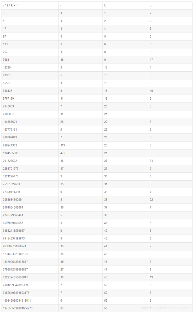
We found that NTT has very strong restrictions on $p$, so it is usually only used in competitions.
## Basic- $\text {VI}$ -Fast Walsh Transform (FWT)
### BVI-1 Bitwise Operators
#### BVI-1-1 Bitwise AND
Bitwise AND, is generally denoted as $\&, \wedge$, or $\operatorname{and}$.
Assuming we have two positive integers $A, B$, we first convert them into binary $(A)_2, (B) _2$. Then, for each bit of the binary number, if the bit of $(A) _2, (B) _2$ is both $1$, then the bit of $(A \&B) _2$ is $1$, otherwise it is $0$.
Example:
$$
100101011100\ \&\ 111000100111 = 100000000100
$$
#### BVI-1-2 Bitwise OR
按位与,又称为按位且,一般记为 $|,\vee$ 或 $\operatorname{or}$。
假设我们有两个正整数 $A,B$,我们先将它转成二进制 $(A)_2,(B)_2$,然后,对于二进制数的每一位,如果 $(A)_2,(B)_2$ 的这一位**都是** $0$,则 $(A|B)_2$ 的这一位是 $0$,否则这一位是 $1$。
例:
Bitwise OR, nerally denoted as $|, \vee$, or $\operatorname{or}$.
Assuming we have two positive integers $A, B$, we first convert them into binary $(A)_2, (B) _2$. Then, for each bit of the binary number, if the bit of $(A) _2, (B) _2$ is both $0$, then the bit of $(A|B) _2$ is $0$, otherwise it is $1$.
Example:
$$
100101011100\ |\ 111000100111 = 111101111111
$$
#### BVI-1-2 Bitwise XOR
按位异或一般记为 $\oplus,^\wedge$ 或 $\operatorname{xor}$。
假设我们有两个正整数 $A,B$,我们先将它转成二进制 $(A)_2,(B)_2$,然后,对于二进制数的每一位,如果 $(A)_2,(B)_2$ 的这一位相同,则 $(A\oplus B)_2$ 的这一位是 $0$,否则这一位是 $1$。
例:
Bitwise XOR is generally denoted as $\oplus, ^\wedge$, or $\operatorname {xor}$.
Assuming we have two positive integers $A, B$, we first convert them into binary $(A) _2, (B) _2$. Then, for each bit of the binary number, if the bits of $(A) _2, (B) _2$ are the same, then the bit of $(A \oplus B) _2$ is $0$, otherwise it is $1$.
Example:
$$
100101011100\ \oplus\ 111000100111 = 011101111011
$$
### BVI-2 Bitwise Convolution
#### BVI-2-1 Definition
我们现在有两个序列 $\{a_n\},\{b_n\}$ (**这里假定序列下标从 $0$ 开始,也就是说最后一项是 $a_{n-1}$**)。
我们定义
$$
\begin{aligned}
\phi_x=\sum_{i\&j=x}a_ib_j\\
\psi_x=\sum_{i|j=x}a_ib_j\\
\xi_x=\sum_{i\oplus j=x}a_ib_j\\
\end{aligned}
$$
此时我们考虑如何快速计算这三个序列的值。
#### BVI-2-2 快速沃尔什变换
##### 按位与卷积
仿照快速傅里叶变换的思路,定义 $\Phi\{a\}$ 是序列 $\{a_n\}$ 经过按位与意义下快速沃尔什变换后的结果。
此时我们希望有 $\Phi\{\phi\}=\Phi\{a\}\times\Phi\{b\}$。
此处 “$\times$” 就是每一项对应相乘。
这一步仅需在 $O(n)$ 的复杂度下从 $0$ 到 $(n-1)$ 依次遍历即可。
所以问题转化成如何构造 $\Phi$,以及如何快速计算 $\Phi\{a\}$。
令 $\Phi\{a\}_x=\displaystyle\sum_{x\&i=x(0\le i<n)}a_i$。
验证:
$$
\begin{aligned}
&\Phi\{a\}_x\times\Phi\{b\}_x\\
=&\left(\sum_{x\&i=x(0\le i<n)}a_i\right)\left(\sum_{x\&j=x(0\le j<n)}b_j\right)\\
=&\sum_{x\&i=x(0\le i<n)}\left(a_i\sum_{x\&j=x(0\le j<n)}b_j\right)\\
=&\sum_{x\&i=x(0\le i<n)}\sum_{x\&j=x(0\le j<n)}a_ib_j\\
=&\sum_{x\&(i\&j)=x(0\le i,j<n)}a_ib_j\\
=&\Phi\{\phi\}_x
\end{aligned}
$$
满足条件。
> **上述步骤中的细节**
> 1. 两个和式乘起来的括号是可以分开的,原因是乘法对加法有分配律,故直接拆开式子即可。
> 2.
> $$
> \begin{cases}x\&i=x\\ x\&j=x\end{cases}\iff x\&(i\&j)
> $$
> 原因是,对于每一个二进制位,如果 $x$ 的这一位是 $1$,那么 $i,j$ 的这一位也必然是 $1$,所以 $i\&j$ 的这一位也一定是 $1$。
> 这两个条件是等价的,所以用“$\iff$”。
快速计算 $\Phi\{a\}$ 的方法依然使用分治思想进行考虑。
依然假定 $n=2^k(k\in\mathbb{N})$。
对于序列的前半段 $\{a_{[0,\frac{n}{2})}\}$,它们的下标的二进制首位是 $0$,对于后半段 $\{a_{[\frac{n}{2},n)}\}$,它们的下标的二进制首位是 $1$。
设 $\{a_{[0,\frac{n}{2}]}\}=\{u\},\{a_{[\frac{n}{2}+1,n)}\}=\{v\}$。
首先我们可以得到 $\Phi\{a\}_i=\Phi\{v\}_i(\frac n 2\le i<n)$,因为对于 $i\&j=i$ 的 $j$ 必定也在 $[\frac{n}{2},n)$ 之间。
但是对于 $0\le i<\frac n 2$ 的 $i$,对应的 $j$ 的范围是没有限制的,所以此时 $\Phi\{a\}_i=\Phi\{u\}_i+\Phi\{v\}_i$。
所以我们有 $\Phi\{a\}=\operatorname{merge}(\Phi\{u\}+\Phi\{v\},\Phi\{v\})$ 。
其中 $\operatorname{merge}$ 为将两个序列拼接。
那么可以递归求解,复杂度 $T(n)=2T(\frac n 2)+O(n)=O(n\log n)$。
##### 按位或卷积
同样的,定义 $\Psi\{a\}$ 是序列 $\{a_n\}$ 经过按位或意义下快速沃尔什变换后的结果。
此时我们希望有 $\Psi\{\psi\}=\Psi\{a\}\times\Psi\{b\}$。
令 $\Phi\{a\}_x=\displaystyle\sum_{x|i=x(0\le i<n)}a_i$。
验证:
$$
\begin{aligned}
&\Psi\{a\}_x\times\Psi\{b\}_x\\
=&\left(\sum_{x|i=x(0\le i<n)}a_i\right)\left(\sum_{x|j=x(0\le j<n)}b_j\right)\\
=&\sum_{x|i=x(0\le i<n)}\left(a_i\sum_{x|j=x(0\le j<n)}b_j\right)\\
=&\sum_{x|i=x(0\le i<n)}\sum_{x|j=x(0\le j<n)}a_ib_j\\
=&\sum_{x|(i|j)=x(0\le i,j<n)}a_ib_j\\
=&\Psi\{\psi\}_x
\end{aligned}
$$
满足条件。
仿照前文,我们有 $\Psi\{a\}=\operatorname{merge}(\Psi\{u\},\Psi\{u\}+\Psi\{v\})$ 。
递归求解,复杂度 $T(n)=2T(\frac n 2)+O(n)=O(n\log n)$。
##### 按位异或卷积
同样的,定义 $\Xi\{a\}$ 是序列 $\{a_n\}$ 经过按位与意义下快速沃尔什变换后的结果。
此时我们希望有 $\Xi\{\xi\}=\Xi\{a\}\times\Xi\{b\}$。
令 $\Xi\{a\}_x=\displaystyle\sum_{x \circ i=0(0\le i<n)}a_i-\displaystyle\sum_{x\circ j=1(0\le j<n)}a_j$。
其中 $x\circ y=x|y$ 的二进制中 $1$ 的数量的奇偶性。
由于有 $(x\circ y)\oplus(x\circ z)=x\circ(y\oplus z)$,所以上式如同前文一样可以验证。
仿照前文,并根据 $\circ$ 的定义,我们有 $\Xi\{a\}=\operatorname{merge}(\Xi\{u\}+\Xi\{v\},\Xi\{u\}-\Xi\{v\})$ 。
其中 $\operatorname{merge}$ 为将两个序列拼接。
递归求解,复杂度 $T(n)=2T(\frac n 2)+O(n)=O(n\log n)$。
#### BVI-2-3 快速沃尔什逆变换
我们希望有 $\Phi^{-1}\{\Phi(a)\}=a,\Psi^{-1}\{\Psi(a)\}=a,\Xi^{-1}\{\Xi(a)\}=a$。
那么,根据前文所推到的式子, 我们很容易有:
1. $\Phi^{-1}\{a\}=\operatorname{merge}(\Phi\{u\}-\Phi\{v\},\Phi\{u\})$
2. $\Psi^{-1}\{a\}=\operatorname{merge}(\Psi\{u\},\Psi\{u\}-\Psi\{v\})$
3. $\Xi^{-1}\{a\}=\operatorname{merge}(\frac{\Xi\{u\}-\Xi\{v\}}{2},\frac{\Xi\{u\}+\Xi\{v\}}{2})$
## Basic- $\text {VII}$ -多项式求逆
### BVII-1 逆元与费马小定理
对于整数 $a,b,p$,若 $ab\equiv1\pmod p$,则称 $a,b$ 互为模 $p$ 意义下的数论逆元。
通常记 $b$ 为 $a^{-1}$,在不严格的情况下亦可记作 $\frac{1}{a}$。
对于数论逆元的计算,通常使用费马小定理:
>
> 若 $p$ 为素数,$\gcd(a,p)=1$,即 $a,p$ 互质(可记做 $a\perp p$),那么 $a^{p}$ 和 $a$ 在模 $p$ 意义下同余。
>
> **证明**
> 可以用数学归纳法证明该结论。
> 对于 $a$ 为 $1$ 的情况,结论显然成立。
> 如果 $a^p\equiv a \pmod p$ 成立,
> 则 $(a+1)^p=\displaystyle\sum_{i=0}^p \binom{p}{i}a^i$。
> 根据组合数的定义,$\dbinom{p}{i}=\dfrac{p!}{i!(p-i)!}$。(本文将始终以 $\binom{n}{m}$ 表示组合数而非 $C_n^m$)
> 由于 $p$ 是素数,那么 $(i!(p-i)!)$ 中一定不含有带 $p$ 的因子,所以分子上的 $p$ 不会被约掉。
> 因此 $\dbinom{p}{i}|p$,因此 $(a+1)^p\equiv a+1 \pmod p$。
> $\square$
既然有了这个结论,我们就有推论 $a^{p-1}\equiv a^{p-2}\times a\equiv 1\pmod p$。
所以 $a^{p-2}$ 是 $a$ 的逆元。
通过快速幂算法可以在 $O(\log P)$ 的复杂度内解决。
### BVII-2 线性求逆元
如果你要求 $x^{-1} \bmod p$,那么让 $p$ 对 $x$ 作带余除法。
设 $p=qx+r$,所以 $qx+r\equiv 0 \pmod p$。
两边同乘 $q^{-1}r^{-1}$ 得 $r^{-1}x+q^{-1}\equiv 0 \pmod p$。
于是有 $r^{-1}x\equiv p-q^{-1} \pmod p$。
所以 $x^{-1}\equiv r^{-1}(p-q^{-1})^{-1}$。
有了这个式子,就可以从 $1^{-1}$ 开始,$O(n)$ 递推,得到从 $1$ 到 $n$ 所有整数的逆元。
### BVII-3 多项式求逆
给定一个 $n$ 次多项式 $f(x)$,试求出 $g(x)$,使得 $f(x)g(x)\equiv 1 \pmod {x^n}$。
首先我们得求出 $h(x)$ ,满足 $f(x)h(x)\equiv 1\pmod{x^{\lceil\frac{n}{2}\rceil}}$
很明显因为 $f(x)g(x)\equiv 1 \pmod {x^n}$,所以 $\forall m\le n,f(x)g(x)\equiv 1 \pmod {x^m}$ 。
所以
$$
f(x)g(x)\equiv 1\pmod{x^{\lceil\frac{n}{2}\rceil}}
$$
做差得到
$$
f(x)(g(x)-h(x))\equiv 0\pmod{x^{\lceil\frac{n}{2}\rceil}}
$$
两边同除去一个 $f(x)$ 得
$$
g(x)-h(x)\equiv 0\pmod{x^{\lceil\frac{n}{2}\rceil}}
$$
两边平方得
$$
g(x)^2-2g(x)h(x)+h(x)^2\equiv 0\pmod{x^{n}}
$$
移项得 $$g(x)^2\equiv 2g(x)h(x)-h(x)^2\pmod{x^{n}}$$ 合并同类项
$$
g(x)^2\equiv h(x)(2g(x)-h(x))\pmod{x^{n}}
$$
两边同除一个 $g(x)$ (模意义下相当于同乘一个 $f(x)$)
$$
g(x)\equiv h(x)(2-h(x)f(x))\pmod{x^{n}}
$$
$h(x)$ 递归继续算即可,$h(x)f(x)$ 可以用 NTT $O(n\log n)$ 解决。
最终递归到 $\bmod x$ 时,$g(x)=[x^0]f(x)^{-1}$。
注意,此时 $[x^0]f(x)$ 不可为 $0$,否则要引入形式 Laurent 级数,后文将会进行详细介绍。
复杂度 $T(n)=T(\frac n 2)+O(n\log n)=O(n\log n)$。
## Basic- $\text {VIII}$ -多项式除法/取模
如果要对多项式进行带余除法(注意是带余除法而不是乘逆元),我们可以进行如下操作:
求出 $f(x)$ 除以 $g(x)$ 的商 $Q(x)$ 和余式 $r(x)$。
设 $f$ 的次数为 $n$,$g$ 的次数为 $m$,则自然有 $Q$ 的次数为 $n-m$,$r$ 的次数不超过 $m-1$。
那么我们可以认定 $r$ 的次数就是 $m-1$,高次项没有就使系数为 $0$ 即可。
定义:
$$
\tilde{F}(x)=x^{c}F(\frac{1}{x})
$$
此处 $c$ 就是 $F$ 的次数。
容易发现上式其实就是 $F$ 的系数翻转的结果。
那么根据式子:$f(x)=Q(x)g(x)+r(x)$,替换 $x$ 为 $\frac 1 x$ 得:
$$
f(\frac 1 x)=g(\frac 1 x)Q(\frac 1 x)+r(\frac 1 x)
$$
等式两边同乘一个 $x^n$ 得:
$$
\begin{aligned}
x^nf(\frac 1 x)&=x^ng(\frac 1 x)Q(\frac 1 x)+x^nr(\frac 1 x)\\
&=x^mg(\frac 1 x)x^{n-m}Q(\frac 1 x)+x^{n-m+1}x^{m-1}r(\frac 1 x)\\
&=\tilde{g}(x)\tilde{Q}(x)+x^{n-m+1}\tilde{r}(x)\\
&=\tilde{f}(x)
\end{aligned}
$$
也就是
$$
\tilde{f}(x)=\tilde{g}(x)\tilde{Q}(x)+x^{n-m+1}\tilde{r}(x)
$$
发现放到模 $x^{n-m+1}$ 意义下可以把 $\tilde{r}(x)$ 项消去。
$$
\tilde{f}(x)\equiv\tilde{g}(x)\tilde{Q}(x)\pmod{x^{n-m+1}}
$$
那 $\tilde{Q}(x)$ 即为 $\tilde{f}(x)\tilde{g}^{-1}(x)$。
做多项式求逆即可得出 $\tilde{Q}(x)$,翻转系数得 $Q(x)$,回代到原式得 $r(x)$。
复杂度依然是 $O(n\log n)$。
## Basic- $\text {IX}$ -形式导数
这里引用 OI-wiki 的一句话:
>
> 尽管一般环甚至未必存在极限,我们依然可以定义形式幂级数的**形式导数**。
>
如果将多项式仍看作与多项式函数等价,那么可能会有不连续或不可导的情况,甚至 $\mathbb{R}$ 上的很多性质都无法满足,但是对于一个普通的多项式,也即一个形式幂级数,我们无需考虑**函数值**的连续性、可导性甚至是敛散性,直接做形式上的导数即可。
可以得到:
$$
\frac{\mathrm d}{\mathrm dx}\sum_{i=0}^{n}a_ix^i=\sum_{i=1}^{n}ia_ix^{i-1}
$$
## Basic- $\text {IX}$ -形式不定积分
我们通常忽略积分结果中的常数项 $C$。
则有:
$$
\int\sum_{i=0}^{n}a_ix^i\mathrm dx=\sum_{i=1}^{n}\frac{a_i}{i}x^i
$$
## Basic- $\text {XI}$ -指数运算
### BXI-1 多项式自然对数
如果我们要求 $\ln(f(x))\bmod x^n$ ,可以用如下方式处理。
根据公式:
$$
\frac{\mathrm d}{\mathrm dx}\ln(x)=\frac{1}{x}
$$
那么由链式求导法则可以得到:
$$
\frac{\mathrm d}{\mathrm dx}\ln(f(x))=\frac{f'(x)}{f(x)}
$$
即为:
$$
\int\frac{f'(x)}{f(x)}\mathrm dx=\ln(f(x))
$$
那么做一遍求逆,再做一遍求导和积分就可以得到。
其实这就是求解分式的不定积分的一种处理方式。
### BXI-2 多项式 $\exp$
定义 $\exp(x):=\mathrm{e}^x$,我们要求出其模 $x^n$ 得到的多项式。
首先说明,若 $f(x)$ 的常数项不是 $0$,那么 $\exp(f(x))$ 不存在。
原因是对它做泰勒展开,或者是说,给出它的指数生成函数:$\mathrm{e}^{f(x)}=\displaystyle\sum_{i\ge 0}\dfrac{f(x)^i}{i!}$,
你会得到 $[x^0]\mathrm{e}^{f(x)}=\displaystyle\sum_{i\ge 0}\dfrac{[x_0]f(x)^i}{i!}$。
而这在模意义下是发散的。
注意,虽然形式幂级数是一个形式符号,不考虑其敛散性,但其常数项依然是一个数域中的元素。
所以 $f(x)$ 的常数项需要为 $0$。
此时取的 $x^n$ 中 $n$ 越大,最终实现的效果越精细,但不会达到最终答案。
关于这方面的拓展知识涉及到 $p$ 进数,域论等相关知识,感兴趣的不妨阅读李白天的 [《无理数取模怎么做?》](https://www.luogu.me/article/mpgzgle2) 。
此处先给出关于多项式 $\exp$ 的常用的计算公式:
设 $E(x)=\exp(f(x))\bmod x^n,E'(x)=\exp(f(x))\bmod \lceil\dfrac{x^n}{2}\rceil$ ,那么有:
$$
E(x)\equiv E'(x)(1-\ln E'(x)+f(x))\pmod {x^n}
$$
这个公式的证明参见后文。
## Basic- $\text {XII}$ -多项式三角函数
根据欧拉公式,我们有 $\mathrm{e}^{\mathrm{i}\theta}=\cos\theta+\mathrm{i}\sin\theta$。
所以进一步我们可以得出 $\mathrm{e}^{-\mathrm{i}\theta}=\cos\theta-\mathrm{i}\sin\theta$。
所以有
$$
\cos\theta=\frac{\mathrm{e}^{\mathrm{i}\theta}+\mathrm{e}^{-\mathrm{i}\theta}}{2}
$$
$$
\sin\theta=\frac{\mathrm{e}^{\mathrm{i}\theta}-\mathrm{e}^{-\mathrm{i}\theta}}{2\mathrm{i}}
$$
直接根据 $\exp$ 计算即可。
还有另外一个要点,通常我们需要得到答案模 $p$ 的结果,否则输出结果可能太大。
为了得到 $\mathrm{i}\bmod p$ 的值,我们可以做 $-1$,也就是 $p-1$ 的二次剩余来得出。
通常,对于 $p=998244353$ 来说,$\mathrm{i}\equiv 86583718$。
对于 $\tan,\cot,\sec,\csc$ 来说,都可以通过 $\cos,\sin$ 互相计算得出。
## Basic- $\text {XIII}$ -多项式开根
注意,显然开根操作会得到两个和为 $0$ 的解,因此在实际应用中,我们通常取常数项较小的解。
(此处感谢 LRC 与 nueryim 学长的提醒)
### BXIII-1 $\exp$ 法
在解决数学题目的过程中,我们常用到这一变换:$a^b=\mathrm{e}^{b\ln(a)}$。
根据此式,则有 $\sqrt{a}=\mathrm{e}^{\frac{\ln(a)}{2}}$。
直接计算即可。
### BXIII-2 倍增法
仿照多项式求逆的思路,我们假定 $g(x)^2\equiv f(x)\pmod{x^n},h(x)^2\equiv f(x)\pmod{x^{\lceil\frac{n}{2}\rceil}}$。
$$
\begin{aligned}
f(x)-h(x)^2&\equiv0\pmod{x^{\lceil\frac{n}{2}\rceil}}\\
(f(x)-h(x)^2)^2&\equiv0\pmod{x^{n}}\\
(f(x)+h(x)^2)^2&\equiv4f(x)h(x)^2\pmod{x^{n}}\\
\left(\frac{f(x)+h(x)^2}{2h(x)}\right)^2&\equiv f(x)\pmod{x^n}\\
\frac{f(x)+h(x)^2}{2h(x)}&\equiv g(x)\pmod{x^n}\\
\end{aligned}
$$
递归向下计算,复杂度 $T(n)=T(\frac{n}{2})+O(n\log n)=O(n\log n)$。
那么,对于最终递归到 $\bmod x$ 时,$g(x)$ 为 $[x_0]f(x)$ 模 $P$ 意义下的二次剩余。
对于二次剩余,常见求法的为 Cipolla 算法,与本文其他部分关系不大,不展开叙述。
## Basic- $\text {XIV}$ -多项式反三角函数
对反三角函数进行求导,可以得到:
$$
\frac{\mathrm{d}}{\mathrm{d}x}\arcsin(x)=\frac{1}{\sqrt{1-x^2}}
$$
故有
$$
\int\frac{1}{\sqrt{1-x^2}}\mathrm{d}x=\arcsin(x)
$$
同理,有:
$$
-\int\frac{1}{\sqrt{1-x^2}}\mathrm{d}x=\arccos(x)
$$
$$
\int\frac{1}{1+x^2}\mathrm{d}x=\arctan(x)
$$
将 $f(x)$ 代入,仍然使用链式求导法则:
$$
\begin{aligned}
\int\frac{f'(x)}{\sqrt{1-f(x)^2}}\mathrm{d}x=\arcsin(f(x))\\
-\int\frac{f'(x)}{\sqrt{1-f(x)^2}}\mathrm{d}x=\arccos(f(x))\\
\int\frac{f'(x)}{1+f(x)^2}\mathrm{d}x=\arctan(f(x))\\
\end{aligned}
$$
这里都属于初步的反函数求导法则,不需要其他分析学技巧。
---
至此,前文所述都属于形式幂级数的基本内容。
# PART 3 —— 进阶多项式算法
## Advanced- $\text {I}$ -牛顿迭代
### AI-1 泰勒公式
$$
f(x)=f (x_0)+f' (x_0)(x-x_0)+\frac{f'' (x_0)}{2!}(x-x_0)^2+\dots+\frac{f^{(n)}(x_0)}{n!}(x-x_0)^n+o ((x-x_0)^n)
$$
其中当 $f(x_0)$ 无穷次可导时,则转 变为泰勒级数:
$$
f(x)=\sum_{i\ge0}\frac{f^{(i)}(x_0)(x-x_0)^i}{i!}
$$
$x_0$ 取 $0$ 时即为麦克劳林级数:
$$
f(x)=\sum_{i\ge0}\frac{f^{(i)}(0)}{i!}x^i
$$
扩展到二元的情况,有:
$$
f(x+\Delta x,y+\Delta y)=\sum_{i\ge 0}\frac{1}{i!}\left(\Delta x\frac{\partial}{\partial x }\Delta y\frac{\partial}{\partial y }\right)^if(x,y)
$$
### AI-2 多项式牛顿迭代
给你一个二元多项式 $G(x,y)$,求出 $G(x,f(x))\equiv0\pmod{x^n}$ 时的 $f(x)$ 的表达式,$f$ 亦为多项式。
其中 $G$ 满足:
+ $\exists \xi,\text{s.t.} G(0,\xi)=0\land\dfrac{\partial G}{\partial y}(0,\xi)\neq0$。
其实后面那个偏导式的意思即为:$G(x,y)$ 在 $x=0$ 时不恒为 $0$。
依然考虑倍增法:
假设 $G(x,g(x))\equiv0\pmod{x^{\lceil\frac{n}{2}\rceil}}$。
将 $G(x,f(x))$ 对在 $f(x)=g(x)$ 处进行泰勒展开,有:
$$
G(x,f(x))=\sum_{i\ge0}\frac{\frac{\partial^iG}{\partial y^i}(x,g(x))}{i!}(f(x)-g(x))^i\equiv0\pmod{x^n}
$$
因为有 $f(x)\equiv g(x)\pmod{x^{\lceil\frac{n}{2}\rceil}}$,所以 $(f(x)-g(x))$ 的最低非零次项至少是 $x^{\lceil\frac{n}{2}\rceil}$。
所以对 $\forall i>1$,都有 $(f(x)-g(x))^i\equiv 0\pmod{x^n}$。
所以原式等价于:
$$
G(x,g(x))+(f(x)-g(x))\frac{\partial G}{\partial y}(x,g(x))\equiv0\pmod{x^n}
$$
移项之后得到:
$$
f(x)\equiv g(x)-\frac{G(x,g(x))}{\frac{\partial G}{\partial y}(x,g(x))}\pmod{x^n}
$$
倍增计算即可。
其实这个式子就是牛顿迭代的式子。
初始条件是,$n=1$ 时,$\xi$ 即为解。
### AI-3 具体应用
这里举几个例子。
#### AI-3-1 多项式求逆
设我们要求出 $F(x)^{-1}$,那么构造 $G(x,y)=y^{-1}-F(x)$。
所以:
$$
f(x)\equiv g(x)-\frac{g(x)^{-1}-F(x)}{-g(x)^{-2}}=2g(x)-F(x)g(x)^{2}=g(x)(2-F(x)g(x))\pmod{x^n}
$$
与之前的推导结果一致。
#### AI-3-2 多项式 $\exp$
构造 $G(x,y)=\ln(y)-F(x)$。
$$
f(x)\equiv g(x)-\frac{\ln(g(x))-F(x)}{g(x)^{-1}}=g(x)(1-\ln(g(x))-F(x))\pmod{x^n}
$$
证明了上一章未证明的公式。
## Advanced- $\text {II}$ -Chirp-Z 变换
考虑 NTT 或 DFT 的过程,都是将原多项式 $f(x)$ 转化为点值表达式,其中点值取单位根或原根的若干次幂。
不妨对该过程进行扩展:考虑任意一个非零数 $c$,求出 $f(c^0),f(c^1),\cdots,f(c^{m-1})$。
首先,有一个显然的引理:$ij=\dbinom{i+j}{2}-\dbinom{i}{2}-\dbinom{j}{2}$。
该引理或许在某些数学题中有一定的用途。
然后得到式子:
$$
\begin{aligned}
f(c^j)&=\sum_{i=0}^{n-1}a_ic^{ij}\\
&=\sum_{i=0}^{n-1}a_ic^{\binom{i+j}{2}-\binom{i}{2}-\binom{j}{2}}\\
&=c^{-\binom{j}{2}}\sum_{i=0}^{n-1}a_ic^{\binom{i+j}{2}-\binom{i}{2}}\\
&=c^{-\binom{j}{2}}\sum_{i=0}^{n-1}\frac{a_i}{\binom{i}{2}}c^{\binom{i+j}{2}}\\
\end{aligned}
$$
设 $u_i=\frac{a_i}{\binom{i}{2}},v_i=c^{\binom{n+m-2-i-j}{2}}$。
则有:
$$
\begin{aligned}
&=c^{-\binom{j}{2}}\sum_{i=0}^{n-1}u_iv_{n+m-2-i-j}\\
&=c^{-\binom{j}{2}}\sum_{x+y=n+m-2-j}u_xv_y\\
&=c^{-\binom{j}{2}}(u*v)_{n+m-2-j}\\
\end{aligned}
$$
如果下标超过了定义域那直接赋 $0$,对于 $(u*v)$ 的计算使用 NTT。
## Advanced- $\text {III}$ -上升幂与下降幂
定义:
$$
x^{\overline{n}}=\displaystyle\prod_{i=0}^{n-1}(x+i)=\frac{(x+n-1)!}{(x-1)!}
$$
$$
x^{\underline{n}}=\displaystyle\prod_{i=0}^{n-1}(x-i)=\frac{x!}{(x-n)!}
$$
此后我们重新规定 $\dbinom{n}{m}=\dfrac{n^{\underline{m}}}{m!}$,不难发现,在 $n\in \mathbb{N}$ 时与原先的定义是等价的,但是该式子可以将组合数直接扩展至 $n\in\mathbb{R}$ 而无需引入 $\Gamma$ 函数。
这样便可以扩展二项式定理至指数为实数的情况,例如 $(a+b)^{\frac{1}{2}}$。
由此进行扩展,不难得出,
负的下降幂即为:
$$
x^{\underline{-n}}=\frac{1}{(x+1)^{\overline{m}}}
$$
负上升幂同理。
## Advanced- $\text {V}$ -分治乘法
对于高次多项式乘低次多项式的情况下,FFT 和 NTT 或许反而不优。
例如,计算 $n$ 次式 $f(x)$ 乘 $1$ 次式 $(ax+b)$ 来说,做 NTT 需要 $O(n\log n)$ 次运算,但是直接计算 $axf(x)+bf(x)$ 只包含数乘以及多项式加法的开销,复杂度被降成 $O(n)$。
此方法只有在另一低次式的项数小于 $\log n$ 时才有效。
不妨进行一些扩展。
若给定 $n$ 个低次多项式 $f_1(x),f_2(x),\cdots,f_n(x)$,求出 $\displaystyle\prod_{i=1}^nf_i(x)$。
朴素的方法是对这些多项式扫一遍,依次用 NTT 进行相乘,复杂度为 $O(n^2\log n)$,无法接受。
根据前文所述方法,直接相乘,可将复杂度降为 $O(n^2)$。
我们假设 $\displaystyle\prod_{i=1}^{\frac{n}{2}}f_i(x),\displaystyle\prod_{i=\frac{n}{2}+1}^nf_i(x)$ 已经计算好了,那么将这两个多项式进行乘法的复杂度是 $O(n\log n)$。
由主定理,该算法的复杂度 $T(n)$ 相当于每次递归拆成两部分,合并复杂度 $O(n\log n)$,总复杂度为 $T(n)=2T(\frac{n}{2})+O(n\log n)=O(n\log^2n)$。
可以接受。
算法的结构如下图所示。
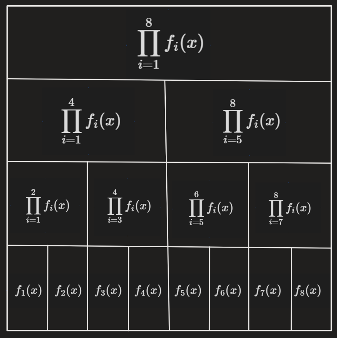
其结构与具体流程类似数据结构线段树。
## Advanced- $\text {IV}$ -多项式平移
其实本质是形式幂级数复合的“弱化版“。
给定一个多项式 $f(x)=\displaystyle\sum_{i=0}^{n-1}a_ix^i$,求出多项式 $f(x+c)$ 。
这里只介绍最快速的方法:二项式定理法。
$$
\begin{aligned}
f(x+c)&=\sum_{i=0}^{n-1}a_i(x+c)^i\\
&=\sum_{i=0}^{n-1}a_i\sum_{j=0}^i\binom{i}{j}x^jc^{i-j}\\
&=\sum_{j=0}^{n-1}x^j\sum_{i=j}^{n-1}\binom{i}{j}a_ic^{i-j}\\
&=\sum_{j=0}^{n-1}x^j\sum_{i=j}^{n-1}\frac{i^{\underline{j}}}{j!}a_ic^{i-j}\\
&=\sum_{j=0}^{n-1}x^j\sum_{i=j}^{n-1}\frac{i!}{j!(i-j)!}a_ic^{i-j}\\
&=\sum_{j=0}^{n-1}\frac{x^j}{j!}\sum_{i=j}^{n-1}i!a_i\frac{c^{i-j}}{(i-j)!}
\end{aligned}
$$
设 $u_i=(n-1-i)!a_{n-1-i},v_i=\dfrac{c^i}{i!}$。
则原式为 $\displaystyle\sum_{j=0}^{n-1}\frac{x^j}{j!}\sum_{i=j}^{n-1}u_{n-1-i}v_{i-j}$。
再化简:
$$
\sum_{j=0}^{n-1}\frac{x^j}{j!}\sum_{x+y=n-1-j}u_{x}v_{y}
$$
于是我们用 NTT 计算 $(u*v)$,翻转后每一位乘上 $(j!)^{-1}$ 即为 $f(x+c)$ 的系数。
## Advanced- $\text {V}$ -插值
在高中数学的数列一章中,我们经常需要根据某个数列的前若干项来计算其通项公式。
一般来说,这些数列的规律都易于观察,例如:${a_n}=\{1,2,4,8,16,32,\cdots\}$,容易观察出其通项公式为 $a_n=2^n$。
那么,机械化的计算机该如何解决此类问题?
或者是,当数列的前若干难以得到简单规律时,该如何得出通项公式?
进一步的,若给出连续函数的某一些点值,如何求出该函数的某一个可能值?
我们需要引入新的公式。
插值,即给定 $n$ 个点值 $x_1,x_2,\cdots,x_n$ 以及 $n$ 个函数值 $y_1,y_2,\cdots,y_n$,求出一个连续函数 $f(x)$,使得:$\forall i\in[1,n]\cap\mathbb{Z},f(x_i)=y_i$。
主要用于将离散的数据连续化以进行估算,在实际生活中应用相对较广。
不难发现,IDFT、INTT 其实就是 $x_i$ 为某些特定数时的插值。
### AV-1 线性插值
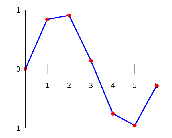
朴素的构造方法是,对于这 $n$ 个点 $(x_1,y_1),(x_2,y_2),\cdots,(x_n,y_n)$,按横坐标排序后,横坐标相邻的两个点连一条线段,左右端点之外的部分随便取。
例如下图:
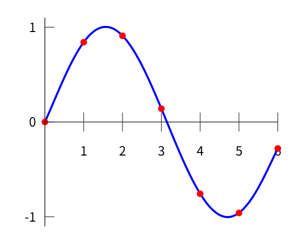
### AV-2 多项式插值
如果需要使得 $f(x)$ 是一个多项式函数,如下图:
直接的想法是构造方程组:
$$
\begin{cases}
a_0+a_1x_1+a_2x_1^2+\cdots+a_{n-1}x_1^{n}=y_1\\
a_0+a_1x_2+a_2x_2^2+\cdots+a_{n-1}x_2^{n}=y_2\\
\quad\quad\quad\quad\quad\quad\quad\quad\quad\vdots\\
a_0+a_1x_n+a_2x_n^2+\cdots+a_{n-1}x_n^{n}=y_n\\
\end{cases}
$$
直接运用高斯消元解决,复杂度 $O(n^3)$ ,过于昂贵,无法接受。
于是我们有拉格朗日插值公式:
$$
f(x)=\sum_{i=1}^{n}y_i\prod_{j\neq i}\frac{x-x_j}{x_i-x_j}
$$
验证:
$$
f(x_c)=\sum_{i=1}^{n}y_i\prod_{j\neq i}\frac{x_c-x_j}{x_i-x_j}
$$
当 $i\neq c$ 时,必有一项的分子是 $(x_c-x_c)$,故后面的连乘式一定为 $0$。
所以只有 $i=c$ 是,后面的连乘式计算结果为 $1$,故答案为 $y_i$,符合要求。
计算的复杂度为 $O(n^2)$。
还有另一种方法称为牛顿插值,支持 $O(n)$ 插入新点,限于篇幅,此处不过多描述。
除多项式插值外,还有三角插值,利用傅里叶级数进行操作,感兴趣的可以自行查阅相关资料或论文。
## Advanced- $\text {VI}$ -连续点值平移
给你 $f(0),f(1),f(2),\cdots,f(n-1)$ 的值,求出 $f(\delta),f(\delta+1),f(\delta+2),\cdots,f(\delta+n-1)$ 的值。
这里仅讨论 $\delta\ge n$ 的情况。
显然的做法是,先进行拉格朗日插值将 $f$ 的表达式求出来,然后对 $c,c+1,\cdots,c+n-1$ 做多点求值。
复杂度瓶颈是拉格朗日插值的 $O(n^2)$,可以用快速插值做到 $O(n\log^2n)$。
这里有一种更快的 $O(n\log n)$ 做法。
首先,仍然根据拉格朗日插值公式有:
$$
f(x)=\sum_{i=0}^{n-1}f(i)\prod_{j\neq i}\frac{x-j}{i-j}
$$
所以平移之后得到:
$$
\begin{aligned}
f(x+\delta)&=\sum_{i=0}^{n-1}f(i)\prod_{j\neq i}\frac{x+\delta-j}{i-j}\\
&=\sum_{i=0}^{n-1}f(i)\frac{\prod_{j\neq i}(x+\delta-j)}{\prod_{j\neq i}(i-j)}\\
&=\sum_{i=0}^{n-1}f(i)\frac{\prod_{j\neq i}(x+\delta-j)}{(-1)^{n-1-i}i!(n-1-i)!}\\
&=\sum_{i=0}^{n-1}f(i)\frac{\prod_{j\neq i}(x+\delta-j)}{(-1)^{n-1-i}i!(n-1-i)!}\\
&=\sum_{i=0}^{n-1}\frac{f(i)(x+\delta)!}{(-1)^{n-1-i}i!(n-1-i)!(x+\delta-n)!(x+\delta-i)}\\
&=\frac{(x+\delta)!}{(x+\delta-n)!}\sum_{i=0}^{n-1}\frac{f(i)}{(-1)^{n-1-i}i!(n-1-i)!(x+\delta-i)}\\
&=\frac{(x+\delta)!}{(x+\delta-n)!}\sum_{i=0}^{n-1}\frac{f(i)}{(-1)^{n-1-i}i!(n-1-i)!}\frac{1}{x+\delta-i}\\
\end{aligned}
$$
设 $u_i=\dfrac{f(i)}{(-1)^{n-1-i}i!(n-1-i)!},v_i=\dfrac{1}{\delta-n+1+i}$,超出定义域设为 $0$。
原式则为:
$$
\begin{aligned}
&=\frac{(x+\delta)!}{(x+\delta-n)!}\sum_{i=0}^{n-1}u_iv_{n-1+x-i}\\
&=\frac{(x+\delta)!}{(x+\delta-n)!}\sum_{i=0}^{n-1+x}u_iv_{n-1+x-i}\\
&=\frac{(x+\delta)!}{(x+\delta-n)!}(u*v)_{n-1+x}\\
\end{aligned}
$$
利用 NTT 做出 $(u*v)$,预处理阶乘并计算即可,复杂度瓶颈在 NTT 为 $O(n\log n)$。
> **预处理**
> 预处理,即为在计算之前就进行的提前处理,如:在 NTT 之前先将从 $1\sim n$ 所有整数的阶乘根据 $n!=n(n-1)!$ 递推全部得到,这样就可以以 $O(n)$ 的时间复杂度计算 $u_i$ 和 $v_i$。
## Advanced- $\text {VII}$ -多项式多点求值
给定 $n$ 次多项式 $f(x)$ 和 $n$ 个数 $a_1,a_2,\cdots,a_n$。
求出 $f(a_1),f(a_2),\cdots,f(a_n)$ 的值。
### AVII-1 多项式取模方法
将这 $n$ 个数分成两部分:
$$
\begin{aligned}
&A_0=\left\{a_1,a_2,\cdots,a_{\lfloor\frac{n}{2}\rfloor}\right\}\\
&A_1=\left\{a_{\lfloor\frac{n}{2}\rfloor+1},\cdots,a_{n-1},a_n\right\}\\
\end{aligned}
$$
构造辅助多项式 $t_0(x)=\displaystyle\prod_{a_i\in A_0}(x-a_i),t_1(x)=\displaystyle\prod_{a_i\in A_1}(x-a_i)$。
很显然,当 $x\in A_0$ 时,$t_0(x)=0$。
对于 $f(x),t_0(x)$ 进行带余除法,得到 $f(x)=t_0(x)Q_0(x)+r_0(x)$。
当 $t_0(x)\neq0$ 时就是正常带余除法,$t_0(x)=0$ 时则有 $f(x)=r_0(x)$。
同理可得当 $x\in A_1$ 时 $f(x)=r_1(x)$。
所以我们将这个问题分治成了两个子问题,即对于 $A_0,A_1$ 中的所有点,分别求出对于 $r_0(x),r_1(x)$ 的值。
也就是说,假设对于次数与点的个数为 $n$ 时,设 $T(n)$ 为多项式多点求值的复杂度,则
$$
T(n)=2T(\frac n 2)+O(n\log n)
$$
在分治的过程中,每次计算的规模减半并执行两次,每次向下递归的复杂度为 $O(n\log n)$ ——这是多项式取模所带来的复杂度。
根据主定理,$T(n)=O(n\log^2n)$。
辅助多项式 $t$ 分治乘法直接得到。
### AVII-2 常数优化
多项式取模的时间复杂度是 $O(n\log n)$,但实际应用中需要进行求逆,翻转等一系列操作,常数开销大,因此可以使用更快捷的方法。
对于数 $a$,我们有 $F(a)=[x^0](F(x)\bmod (x-a))$。
考虑快速计算 $F(x)$ 对 $(x-a_1),(x-a_2),\cdots,(x-a_n)$ 取模的结果。
设 $D_a(x)=x-a$,做带余除法得到 $F(x)=D_a(x)Q_a(x)+r$。
注意到 $r$ 仅与 $[x_0]F(x),[x_0]D_a(x),[x_0]Q_a(x)$ 有关,而 $[x_0]F(x),[x_0]D_a(x)$ 是已知的,因此问题被规约为快速计算 $[x_0]Q_a(x)$。
设 $D_{[l,r]}=\displaystyle\prod_{i=l}^r(x-a_i)$,$Q_{[l,r]}$ 为 $F(x)$ 对 $D_{[l,r]}$ 做带余除法得到的商式。
根据多项式除法的公式,在本问题中的描述即为:
$$
\begin{aligned}
\tilde{F}(x)\equiv\tilde{D}_{[l,r]}(x)\tilde{Q}_{[l,r]}(x)\pmod{x^{n-r+l}}\\
\tilde{F}(x)\tilde{D}^{-1}_{[l,r]}(x)\equiv\tilde{Q}_{[l,r]}(x)\pmod{x^{n-r+l}}\\
\end{aligned}
$$
根据分治乘法,定义 $m=\frac{l+r}{2}$,此处默认为下取整。
由于有 $\tilde{D}_{[l,r]}(x)=\tilde{D}_{[l,m]}(x)\tilde{D}_{[m+1,r]}(x)$,所以推论有 $\tilde{D}^{-1}_{[l,m]}(x)=\tilde{D}^{-1}_{[l,r]}(x)\tilde{D}_{[m+1,r]}(x),\ \tilde{D}^{-1}_{[m+1,r]}(x)=\tilde{D}^{-1}_{[l,r]}(x)\tilde{D}_{[l,m]}(x)$。
因此有:
$$
\begin{aligned}
\tilde{Q}_{[l,m]}(x)&\equiv\tilde{F}(x)\tilde{D}^{-1}_{[l,m]}(x)\pmod{x^{n-m+l}}\\
&\equiv\tilde{F}(x)\tilde{D}^{-1}_{[l,r]}(x)\tilde{D}_{[m+1,r]}(x)\pmod{x^{n-m+l}}\\
&\equiv\tilde{Q}_{[l,r]}(x)\tilde{D}_{[m+1,r]}(x)\pmod{x^{n-m+l}}\\
\end{aligned}
$$
同理亦有:
$$
\begin{aligned}
\tilde{Q}_{[m+1,r]}(x)&\equiv\tilde{Q}_{[l,r]}(x)\tilde{D}_{[l,m]}(x)\pmod{x^{n-r+m-1}}\\
\end{aligned}
$$
$\tilde{{D}}^{-1}$ 可以分治乘法预处理。
根据递归式,一直计算下去直到得出 $\tilde{Q}_{a}(x)$ 的常数项即可(或者直接是其本身,因为它是一个零次多项式)。
复杂度没有变化,仍然是 $O(n\log^2 n)$,但每次向下递归从取模变了乘法,常数减小很多。
由于只有 $[x^0]Q_{[l,r]}(x)$,即 $[x^{r-l}]\tilde{Q}_{[l,r]}(x)$ 有用,又因为 $\tilde{Q}_{[l,r]}(x)$ 之后只会乘以次数小于等于 $(r−l)$ 的多项式,也就是说,只需要保留 $\tilde{Q}_{[l,r]}(x)$ 最高的 $(r-l)$ 位即可。
注意,由于 $\tilde{Q}$ 是 $Q$ 取反的结果,所以保留最高的 $(r-l)$ 位后不可在低次项补 $0$,而是直接截断后 $(r-l)$ 位然后形成一个新多项式。
与该方法等价的是应用转置原理(即 Tellegen 定理),根据 $a_1,a_2,\cdots,a_n$ 构成的范德蒙德矩阵进行递归求解。
具体参考陈宇在 2020 年国家集训队论文中的《转置原理的简单介绍》。
## Advanced- $\text {VIII}$ -快速插值
根据前文所述,朴素的拉格朗日插值的时间复杂度为 $O(n^2)$。
这里介绍一种更加快速的处理插值的算法,多项式快速插值。
回顾拉格朗日插值公式:
$$
f(x)=\sum_{i=1}^{n}y_i\prod_{j\neq i}\frac{x-x_j}{x_i-x_j}
$$
设 $t(x)=\displaystyle\prod_{i=1}^n(x-x_i)$。
于是 $\dfrac{t(x)}{x-x_i}=\displaystyle\prod_{j\neq i}(x-x_j)$。
我们发现,当 $x\to x_i$ 时,原式的极限则为 $\displaystyle\prod_{j\neq i}(x_i-x_j)$。
根据洛必达法则,$\displaystyle\prod_{j\neq i}(x_i-x_j)=\displaystyle\lim_{x\to x_i}\dfrac{t(x)}{x-x_i}=\displaystyle\lim_{x\to x_i}\dfrac{t'(x)}{1}=t'(x_i)$。
所以以 $O(n)$ 的时间复杂度对 $t(x)$ 求导即可得出 $\displaystyle\prod_{j\neq i}(x_i-x_j)$。
另一个证明方法是,根据数学归纳法容易得出扩展的求导乘法公式:
$$
\frac{\mathrm d}{\mathrm dx}\prod_{i=1}^nf_i(x)=\sum_{i=1}^nf_i'(x)\prod_{j\neq i}f(j)
$$
根据此公式直接可证明结论。
于是我们有
$$
f(x)=\sum_{i=1}^{n}\frac{y_i}{t'(x_i)}\prod_{j\neq i}(x-x_j)
$$
但是这仍然是 $O(n^2)$,继续优化,考虑拆分:
$f_l(x)=\displaystyle\sum_{i=1}^{\lfloor\frac{n}{2}\rfloor}\frac{y_i}{t'(x_i)}\prod_{j\neq i,j\le \lfloor\frac{n}{2}\rfloor}(x-x_j),f_r(x)=\displaystyle\sum_{i=\lfloor\frac{n}{2}\rfloor+1}^{n}\frac{y_i}{t'(x_i)}\prod_{j\neq i,j> \lfloor\frac{n}{2}\rfloor}(x-x_j)$。
以及 $t_l(x)=\displaystyle\prod_{i=1}^{\lfloor\frac{n}{2}\rfloor}(x-x_i),t_r(x)=\displaystyle\prod_{i=\lfloor\frac{n}{2}\rfloor+1}^{n}(x-x_i)$ 。
递归到底层时,我们需要计算 $\frac{y_i}{t'(x_i)}$ 的值,对于分母 $t'(x_i)$,多点求值进行预处理即可,复杂度 $O(n\log^2n)$。
则有 $f(x)=f_l(x)t_r(x)+f_r(x)t_l(x)$,分治计算,复杂度 $T(n)=2T(\frac{n}{2})+O(n\log n)=O(n\log^2n)$。
# PART 4 —— 高阶多项式技巧
## Senior- $\text {I}$ -拉格朗日反演
### SI-1 形式 Laurent 级数
回顾形式幂级数求逆的过程,只有当 $[x^0]f(x)$ 非零时,$f^{-1}(x)$ 才存在。
如果我们想要计算 $(x^4+x^3)$ 的逆,可以将其因式分解成:$x^3(x+1)$,再进行求逆,得到 $x^{-3}(x+1)^{-1}$。
$(x+1)^{-1}$ 是可求的,然而我们无法以形式幂级数的形式处理 $x^{-3}$。
因此,不妨直接对形式幂级数进行扩展。
先考察数域 $\mathbb{F}$ 上的形式幂级数的定义:集合 $P=\left\{\displaystyle\sum_{i\ge 0}a_ix^i|a_i\in\mathbb{F}\right\}$ 中的元素。
$\mathbb{F}[[x]]$ 即为 $(P,+,\times)$。
定义数域 $\mathbb{F}$ 上的形式 Laurent 级数为集合 $L=\left\{\displaystyle\sum_{i\ge \beta}a_ix^i|a_i\in\mathbb{F},\beta\in\mathbb{Z}\right\}$。
其中文译名为洛朗级数。
对于一个形式 Laurent 级数 $f$,定义 $\operatorname{ord} f$ 为 $f$ 的最低非零次项。
注意,$\operatorname{ord} f$ 不一定与 $\beta$ 相等,因为 $a_i$ 有可能为 $0$。
通俗地讲,形式幂级数即为形式 Laurent 级数在最低次大于等于 $0$ 的子集。
形式 Laurent 级数环记作 $\mathbb{F}((x))$。
根据定义,$\mathbb{F}[[x]],\mathbb{F}((x))$ 都是整环。
#### SII-1-1 加法
形式 Laurent 级数的加(减)法亦为同项相加,即:
$$
h=f+g=\sum_{i\ge\max(\operatorname{ord }f,\operatorname{ord }g)}(a_i+b_i)x^i
$$
#### SII-1-2 乘法
若 $h=fg$,则 $\operatorname{ord }h=\operatorname{ord }f+\operatorname{ord }g$。
$$
h=\left(\sum_{i\ge\operatorname{ord}f}a_ix^i\right)\left(\sum_{i\ge\operatorname{ord}g}b_ix^i\right)
$$
仿照形式幂级数的乘法,化简,最终得到:
$$
h=\sum_{s>\operatorname{ord}f+\operatorname{ord}g}\sum_{i+j=s}a_ib_jx^{s}
$$
其实算是一种广义上的卷积。
形式 Laurent 级数的形式导数与复合与形式幂级数相差不大。
### SI-2 形式留数
定义:对于一个形式 Laurent 级数 $f$,$\operatorname{res} f:=[x^{-1}]f$。
即 $f$ 的 $-1$ 次项。
需要提前明确的是,**形式留数具有线性性**。
同时,形式留数还有一些常用性质。
---
例如,对 $\forall f\in\mathbb{F}((x)),\operatorname{res} f'=0$。
这个性质是平凡的。
---
其根据形式导数进行引申的的性质很丰富。
下式是关于导数乘积法则的性质。
$$
\forall f,g\in\mathbb{F}((x)),\operatorname{res}(fg')=-res(f'g)
$$
证明较为容易: $\operatorname{res}((fg)')=0=\operatorname{res}(fg'+f'g)=\operatorname{res}(fg')+\operatorname{res}(f'g)$。
最后一步根据形式留数的线性性进行推导。
---
其他性质如:
$$
\operatorname{res}\frac{f'}{f}=\operatorname{ord}f
$$
证明考虑直接将分子和分母展开,约分即可。
---
最后是一条重要的公式:
$$
\forall f\in\mathbb{F}((x)),g\in\mathbb{F}[[x]],\operatorname{res}((f\circ g)\times g')=\operatorname{res} f\operatorname{ord}g
$$
注意,形式幂级数的 $\operatorname{ord}$ 也是其最低非零次项。
证明:
因为形式留数具有线性性,所以仅需考虑 $f=x^n$ 的情况。
分类讨论,首先考虑 $n\neq -1$ 的情况。
$$
\begin{aligned}
&\operatorname{res}(g^{n}g')\\
=&\operatorname{res}(\frac{1}{n+1}(g^{n+1})')\\
=&\frac{1}{n+1}\operatorname{res}((g^{n+1})')\\
=&0
\end{aligned}
$$
再考虑 $n=-1$ 的情况。
$$
\begin{aligned}
&\operatorname{res}(\frac{g'}{g})\\
=&\operatorname{ord}g\\
=&\operatorname{res}f\operatorname{ord}g
\end{aligned}
$$
于是原结论证毕。
### SI-3 拉格朗日反演
首先给出一个引理:
对于一个形式 Laurent 级数 $F$,若 $[x^0]F=0,[x^1]F\neq 0$,则必定存在形式 Laurent 级数 $G$,使得 $F\circ G=x$,此时 $G$ 则为 $F$ 的**复合逆**,记作 $F^{\langle-1\rangle}$。
> **关于复合逆**
> 注意到复合逆的定义是 $F\circ G=x$ 而非 $F\circ G=1$,首先这是因为如果条件是 $F\circ G=1$,不难证明只有 $[x^0]F=1$ 时具有唯一平凡解,即 $G=0$,显然没有讨论价值。
> 同时,对于复合运算来说,其构成的幺半群 $(\mathbb{F}((x)),\circ)$ 的单位元为恒等映射 $x$,此时可称为 $\mathrm{id}$,而非 “$1$ “。
根据以上引理,可以得出常见的 $4$ 个版本的拉格朗日反演,这里假定 $G=F^{\langle -1 \rangle}\in \mathbb{F}((x)),\Lambda\in\mathbb{F}((x))$:
$$
\begin{aligned}
&n[x^n]F^k=k[x^{-k}]G^{-n}\\
&n[x^n](\Lambda\circ F)=[x^{n-1}]\frac{\mathrm{d}\Lambda}{\mathrm{d}x}(\frac{x}{G})^n\\
&—————————————\\
&[x^n]F^k=[x^{-k-1}]\frac{\mathrm{d}G}{\mathrm{d}x}G^{-n-1}\\
&[x^n](\Lambda\circ F)=[x^{n}]\Lambda\frac{\mathrm{d}G}{\mathrm{d}x}(\frac{x}{G})^{n+1}\\
\end{aligned}
$$
此处仅证明公式 $2$,其为公式 $1$ 的推广:
**【Format 2】**
$$
\begin{aligned}
\Rightarrow&\Lambda\circ (F\circ G)=\Lambda\\
\Rightarrow&(\Lambda\circ F)\circ G=\Lambda\\
\Rightarrow&(\frac{\mathrm{d}(\Lambda\circ F)}{\mathrm{d}x}\circ G)\frac{\mathrm{d}G}{\mathrm{d}x}=\frac{\mathrm{d}\Lambda}{\mathrm{d}x}\\
\Rightarrow&\frac{\mathrm{d}G}{\mathrm{d}x}\sum_{i=0}^{\infty}[x^i]\frac{\mathrm{d}(\Lambda\circ F)}{\mathrm{d}x}G^i=\frac{\mathrm{d}\Lambda}{\mathrm{d}x}\\
\Rightarrow&\frac{\mathrm{d}G}{\mathrm{d}x}\sum_{i=0}^{\infty}[x^i]\frac{\mathrm{d}(\Lambda\circ F)}{\mathrm{d}x}G^{i-n}=G^{-n}\frac{\mathrm{d}\Lambda}{\mathrm{d}x}\\
\Rightarrow&\sum_{i=0}^{\infty}[x^i]\frac{\mathrm{d}(\Lambda\circ F)}{\mathrm{d}x}G^{i-n}\frac{\mathrm{d}G}{\mathrm{d}x}=G^{-n}\frac{\mathrm{d}\Lambda}{\mathrm{d}x}\\
\Rightarrow&\operatorname{res}\left(\sum_{i=0}^{\infty}[x^i]\frac{\mathrm{d}(\Lambda\circ F)}{\mathrm{d}x}G^{i-n}\frac{\mathrm{d}G}{\mathrm{d}x}\right)=\operatorname{res}\left(G^{-n}\frac{\mathrm{d}\Lambda}{\mathrm{d}x}\right)\\
\Rightarrow&\sum_{i=0}^{\infty}[x^i]\frac{\mathrm{d}(\Lambda\circ F)}{\mathrm{d}x}\operatorname{res}\left(G^{i-n}\frac{\mathrm{d}G}{\mathrm{d}x}\right)=\operatorname{res}\left(G^{-n}\frac{\mathrm{d}\Lambda}{\mathrm{d}x}\right)\\
\Rightarrow&\sum_{i=0}^{\infty}[x^i]\frac{\mathrm{d}(\Lambda\circ F)}{\mathrm{d}x}[i-n=-1]=\operatorname{res}\left(G^{-n}\frac{\mathrm{d}\Lambda}{\mathrm{d}x}\right)\\
\Rightarrow&[x^{n-1}]\frac{\mathrm{d}(\Lambda\circ F)}{\mathrm{d}x}=[x^{-1}]\left(G^{-n}\frac{\mathrm{d}\Lambda}{\mathrm{d}x}\right)\\
\Rightarrow&[x^{n-1}]\frac{\mathrm{d}(\Lambda\circ F)}{\mathrm{d}x}=[x^{n-1}]\frac{\mathrm{d}\Lambda}{\mathrm{d}x}(\frac{x}{G})^n\\
\Rightarrow&[x^{n-1}]\frac{\mathrm{d}(\Lambda\circ F)}{\mathrm{d}x}=[x^{n-1}]\frac{\mathrm{d}\Lambda}{\mathrm{d}x}(\frac{x}{G})^n\\
\Rightarrow&n[x^{n}]\Lambda\circ F=[x^{n-1}]\frac{\mathrm{d}\Lambda}{\mathrm{d}x}(\frac{x}{G})^n\\
\end{aligned}
$$
最后一步基于形式 Laurent 级数复合形式 Laurent 级数仍然是形式 Laurent 级数以及其形式导数的定义而得出。
但是,上面的式子在 $n=0,k<0$ 时无法给出常数项的值,因此拓展到公式 $3,4$。
其证明过程与公式 $2$ 证明过程类似。
## Senior- $\text {II}$ -常系数齐次线性递推
### SII-1 斐波那契数列快速递推
注意,与一般的定义不同,我们认为数列 $\{a_n\}$ 的首项为 $a_0$。
故此处假定斐波那契数列斐波那契数列的前两项为 $f_0=0,f_1=1$,递推公式为:$f_i=f_{i-1}+f_{i-2}$。
如果我们要计算 $f_n$,直接的方法是通过递推式逐一向后递推,复杂度为 $O(n)$。
根据矩阵乘法公式,若矩阵 $C=A\times B$,则:
$$
C_{ij}=\sum_{k=1}^nA_{ik}B_{kj}
$$
因此可以得出:
$$
\begin{bmatrix}
f_{i}\\f_{i-1}
\end{bmatrix}
\begin{bmatrix}
1 & 1\\
1 & 0\\
\end{bmatrix}
=
\begin{bmatrix}
f_{i+1}\\f_{i}
\end{bmatrix}
$$
所以:
$$
\begin{bmatrix}
f_{n+1}\\f_{n}
\end{bmatrix}=
\begin{bmatrix}
1 \\ 0\\
\end{bmatrix}
\begin{bmatrix}
1 & 1\\
1 & 0\\
\end{bmatrix}^{n}
$$
第二个问题是,考虑如何快速计算 $\begin{bmatrix}1 & 1\\1 & 0\\\end{bmatrix}^{n}$。
直接相乘的复杂度是 $O(n)$。
考虑优化,对于任意底数 $a$(不要求是数域中的元素), $a^{n}=(a^{\frac{n}{2}})^2\times a^{n\bmod 2}$,根据该式递归求解,由于平方可以 $O(1)$ 求解,因此每次递归问题规模就被缩小一半,一共最多递归 $O(\log n)$ 次,故时间复杂度为 $O(\log n)$。
由于 $k$ 阶矩阵乘法的复杂度是 $k^3$,因此计算 $f_n$ 的复杂度即为 $O(k^3\log n),k=2$。
这是 $k=2$ 的情况。
考虑一般情况,若一个数列 $f$ 满足 $f_i=\displaystyle\sum_{j=1}^dc_jf_{i-j}$,给定 $f_0,f_1,f_2,\cdots,f_{d-1}$,如何快速求出 $f_n(n\ge d)$?
注意,此时我们称 $f$ 为一个**常系数齐次线性递推数列**。
若依然沿用矩阵乘法,当 $d$ 过大时,复杂度将无法接受。
### SII-2 Fiduccia 算法
#### SII-2-1 特征多项式
我们记一个 $n\times n$ 的矩阵 $A$ 的特征多项式为 $p_A(x)$。
其定义为 $x\mathrm{I}_n-A$ 的行列式的值,其中 $\mathrm{I}_n$ 为 $n$ 阶单位矩阵。
即为:
$$
p_A(x)=\det(x\mathrm{I}_n-A)=
\begin{vmatrix}
x-a_{11}&-a_{12}&\cdots&-a_{1n}\\
-a_{21}&x-a_{22}&\cdots&-a_{2n}\\
\vdots&\vdots&&\vdots\\
-a_{n1}&-a_{n2}&\cdots&x-a_{nn}\\
\end{vmatrix}
$$
需要注意的是,$x$ 既可以是普通多项式中的“形式记号”,也可以是一个矩阵,它只是一个**参量**。
通常来说,这里的 $x$ 应当用 $\lambda$,为了更清晰地体现其多项式性质,此处仍然使用 $x$。
#### SII-2-1 Cayley-Hamilton 定理(C-H 定理)
##### 表述
实际上表述很简单:对于任意的 $n\times n$ 的矩阵 $A$,都有 $p_A(A)=0$。
**容易形成的错误是**,当代入到特征多项式的定义式,即:$\det(A\mathrm{I}_n-A)$ 时,将 $A\mathrm{I}_n$ 看作是矩阵乘法,于是 $\det(A\mathrm{I}_n-A)=\det(A-A)=\det(0)=0$,看起来是一个平凡结论。
实际上,该定理并不平凡,我们需要将 $A\mathrm{I}_n$ 看作是**标量乘法**,而非矩阵乘法,同时,如果参量为矩阵,最终得到的 $0$ 应当表述为 “$\textbf{0}$”,即零矩阵,而非标量 $0$。
换句话说,在最后计算多项式值之前,矩阵 $A$ 是与一个正常的形式记号 $x$ 无异的。
例如,对于矩阵 $A=\begin{bmatrix}a&b\\c&d\end{bmatrix}$ 来说,$p_A(A)$ 应当是:
$$
\begin{aligned}
&p_A(A)\\
=&\det(A\mathrm{I}_n-A)\\
=&\begin{vmatrix}
A-a&-b\\
-c&A-d
\end{vmatrix}\\
=&\begin{vmatrix}
\begin{bmatrix}a&b\\c&d\end{bmatrix}-a&-b\\
-c&\begin{bmatrix}a&b\\c&d\end{bmatrix}-d
\end{vmatrix}\\
=&A^2-(a+d)A+(ad-bc)\mathrm I\\
=&\begin{bmatrix}a^2+bc&ab+bd\\ac+cd&cb+d^2\end{bmatrix}-\begin{bmatrix}a^2+ad&ab+bd\\ac+cd&ad+d^2\end{bmatrix}+
\begin{bmatrix}ad-bc&0\\0&a-bc\end{bmatrix}\\
=&\begin{bmatrix}0&0\\0&0\end{bmatrix}
\end{aligned}
$$
注意,矩阵多项式的常数项中应当有单位矩阵 $\mathrm{I}$ 因子,代表 $n\times m$ 矩阵乘法群的单位元,或 $A^0$,不可忽略,否则矩阵与标量的加减法无法定义。
##### 证明前置定义
**【伴随矩阵】**
在证明之前,仍需要一些定义:
首先定义一个 $n$ 阶矩阵 $K$ 的伴随矩阵 $K^*$ 为:
$$
\begin{bmatrix}
A_{11}&A_{21}&\cdots &A_{n1}\\
A_{12}&A_{22}&\cdots &A_{n2}\\
\vdots&\vdots&&\vdots\\
A_{1n}&A_{2n}&\cdots &A_{nn}\\
\end{bmatrix}
$$
其中 $A_{ij}$ 为 $K$ 的 $(i,j)$ 元的代数余子式,定义为 $(-1)^{i+j}M_{ij}$,即原矩阵划去第 $i$ 行和第 $j$ 列后构成的矩阵的行列式乘 $(-1)^{i+j}$。
**【矩阵多项式】**
注意,矩阵多项式为**系数**是矩阵的多项式,不要混淆。
如果一个矩阵 $A$ 中的每一个元素都是关于 $\lambda$ 的多项式,则 $A$ 必然可以被表示成:
$$
\sum_{i=0}^dA_i\lambda^i
$$
$A_0,A_1,\cdots,A_n$ 即为该矩阵多项式的系数,$d$ 为这些多项式中最高次项次数的最大值。
不难证明,这样的分解是唯一的。
##### 证明
正式开始证明:
设 $W(x)$ 为 $x\mathrm{I}-A$ 的伴随矩阵。
我们假定 $A$ 是 $n$ 阶矩阵。
将 $W(x)$ 写成矩阵多项式的形式,则有 $W(x)=\displaystyle\sum_{i=0}^{n-1}W_ix^i$。
最高次项显然为 $n-1$,因为 $W(x)$ 中的元素都是 $n$ 阶矩阵的代数余子式,少了一行和一列。
由此得式:
$$
\begin{aligned}
&W(x)(x\mathrm{I}-A)\\
=&\sum_{i=0}^{n-1}(W_ix^{i+1}-AW_ix^{i})\\
=&W_{n-1}x^n+\sum_{i=1}^{n-1}(W_{i-1}-AW_{i})x^i-AW_0
\end{aligned}
$$
不妨同时设 $p_A(x)=\displaystyle\sum_{i=0}^n a_ix^i$。
将其转为矩阵,即为 $p_A(x)\mathrm{I}=\displaystyle\sum_{i=0}^n a_ix^i\mathrm{I}$。
根据伴随矩阵的母公式,即 $AA^*=\det(A)\mathrm{I}$ ,可得,$W(x)(x\mathrm{I}-A)=\det(x\mathrm{I}-A)\mathrm{I}=p_A(x)I$。
母公式的证明直接代入矩阵乘法公式,根据行列式按行/列展开的公式易证。
因此我们有:
$$
W_{n-1}x^n+\sum_{i=1}^{n-1}(W_{i-1}-AW_{i})x^i-AW_0=\sum_{i=0}^n a_ix^i\mathrm{I}
$$
并且由于特征多项式一定是首一多项式,即 $a_n=1$,可得:
$$
\begin{bmatrix}
W_{n-1}\\
W_{n-2}-AW_{n-1}\\
W_{n-3}-AW_{n-2}\\
\vdots\\
W_{1}-AW_{2}\\
W_{0}-AW_1\\
AW_0
\end{bmatrix}
=
\begin{bmatrix}
\mathrm{I}\\
a_{n-1}\mathrm{I}\\
a_{n-2}\mathrm{I}\\
\vdots\\
a_2\mathrm{I}\\
a_1\mathrm{I}\\
a_0\mathrm{I}
\end{bmatrix}
$$
对于第 $i$ 行右乘 $A^{n-i+1}$ 得到:
$$
\begin{bmatrix}
W_{n-1}A^n\\
W_{n-2}A^{n-1}-A^nW_{n-1}\\
W_{n-3}A^{n-2}-A^{n-1}W_{n-2}\\
\vdots\\
W_{1}A^2-A^3W_{2}\\
W_{0}A-A^2W_1\\
AW_0
\end{bmatrix}
=
\begin{bmatrix}
A^n\\
a_{n-1}A^{n-1}\\
a_{n-2}A^{n-2}\\
\vdots\\
a_2A^2\\
a_1A\\
a_0\mathrm{I}
\end{bmatrix}
$$
发现等号左边所有值相加为 $\textbf{0}$,右边所有值相加为 $p_A(A)$。
得证。
#### SII-2-3 Fiduccia 算法
该算法在网络上可以找到大量的不严格的,感性化的证明。
对于常系数齐次线性递推数列 $f$ 来说,其转移式为:
$$
\begin{bmatrix}
f_{d-1}\\
f_{d-2}\\
\vdots\\
f_2\\
f_1\\
f_0\\
\end{bmatrix}
\begin{bmatrix}
c_1&c_2&c_3&\cdots&c_{d-1}&c_d\\
1&0&0&\cdots&0&0\\
0&1&0&\cdots&0&0\\
0&0&1&\cdots&0&0\\
\vdots&\vdots&\vdots&&\vdots&\vdots\\
0&0&0&\cdots&1&0\\
\end{bmatrix}^n
=\begin{bmatrix}
f_{n+d-1}\\
f_{n+d-2}\\
\vdots\\
f_n+2\\
f_n+1\\
f_n\\
\end{bmatrix}
$$
记上式中的转移矩阵为 $A$
# PART 5 —— 形式幂级数算法扩展
# PART 6 —— 多项式相关应用
参考资料:
丘维声——《高等代数》
杨一龙——《数学在哪里》
刘承奥——《浅谈DFT在信息学竞赛中的应用》
陈宇——《转置原理的简单介绍》
吕凯风——《集合幂级数的性质与应用及其快速算法》
[OI-wiki](https://oi-wiki.org) ——“多项式与生成函数”部分
Poly Family Bucket (English Version)
https://cwhirly.github.io/2026/03/01/OI/Poly/Poly Family Bucket (English Version)/